3D-1D Coupling
Abstract
Due to the rapid growth of computer technology in the last ten years, it would seem that the finite element method should have grown much more than it did in terms of usage and understanding within the world's engineering and applied science communities.
In order to use the finite element method efficiently and accurately, a considerable amount of idealisation or pre-processing is required. Idealisation is the process of regenerating a geometric model (typically a proposed engineering component created in a computer aided design packages) into an analysis model of suitable quality & reduced size so that it maybe analysed efficiently using the finite element method. Manual idealisation is a specialist skill and is extremely time consuming. Before the finite element method can be used routinely among those working in engineering and the applied sciences, idealisation must be automated.
In recent years several methods of idealising finite element models have emerged. However many cases which would contribute to total idealisation and automation have yet to be considered. Here one such case is discussed, namely the coupling of one dimensional beam elements (suitable for modelling long slender parts of the structure) to three dimensional elements (which are used to represent areas of stress concentration such as joints). The essence of the problem is to ensure compatibility of the displacements at the interface. This is achieved by equating the work done at the dimensional interface by the 3D nodes with the work done at the 1D node. The coupling is then carried out in a manner similar to that used in the development of Reissner plate theory and leads to 6 multi-point constraint equations, one for each degree of freedom of the node in the 1D element. The methods used to achieve the coupling for axial force, bending moment, shear force and torsion are discussed and it is shown that the technique does not introduce any spurious stresses at the dimensional interface.
This new procedure greatly facilitates mixed-dimensional modelling. 3D details such as joints, changes in section or loading are properly represented but dimensionally-reduced beam elements are used to economically and accurately model slender parts, where 3D elements are expensive and potentially ill-conditioned (mathematically unsuitable). Tests on sample structural models show that analysis times can be dramatically reduced when these ideas are implemented.
Introduction
The areas of application and the potential of the finite element method are enormous. Since it's inception in the 1950's, it has developed to be the most powerful tool used in the solution of partial differential equations, which occur in almost all of the applied sciences and engineering fields. It's development has not been paralleled by any other numerical analysis procedure and it has made many other numerical analysis techniques and experimental testing methods redundant. However, despite the time and money invested in an effort to mature the method, there are many avenues to be explored before the method's true elegance and utility is exploited.
The time taken to achieve equilibrium for any given analysis is a function of the number of degrees of freedom (DOF) of the model being analysed. Therefore, if the DOF used to model a particular problem can be reduced while maintaining the same accuracy of the results, an important step in the development of the method has been achieved. Any steps that involve converting the complex real object geometry & loading to a more efficient finite element model (and hence reducing the number of DOF to be solved for) are known as idealisation.
NAFEMS [1] suggests the following categories of idealisation:
MATHEMATICAL MODEL SELECTION
Behavioural assumptions introduced in order to yield a solvable set of expressions but having the side effect of introducing approximations. An example of this is assuming linear elastic behaviour in the finite element method.
PHYSICAL SCALES
Behavioural considerations at different size scales but critical to the prediction of behaviour at all scales. For example, composite materials and soils, where the micro-mechanical behaviour of the individual constituents determines the overall behaviour of the material.
SYMMETRY
By taking advantage of the reflective, rotational or translational symmetry within a component, only part of the component need be modelled, so long as appropriate constraints are applied along the symmetry lines.
DOMAIN SPECIFICATION OR SPATIAL EXTENT
The domain over which the mathematical model is applied. Domain idealisation focuses on a particular area of the model to be analysed and establishes the boundary condition locations e.g. sub-modelling. Figure 1 below shows an example of an analysis which employs sub-modelling.
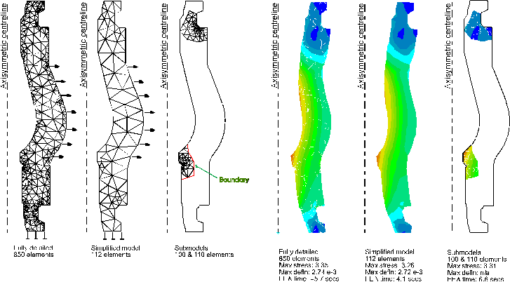
Figure 1: Example of sub-modelling of an oil valve section
Sub-modelling is used to study a local part of a model where the geometric details are small relative to the overall model size. This yields the effects of small details on the stress patterns, without a large number of elements being used. In sub-modelling, an initial course mesh is created on the complete model, and a solution is obtained for the applied loads and constraints. The area of interest is then modelled with a much finer mesh, using results from the coarse model analysis to load the internal boundary of the sub-model.
DETAIL REMOVAL
During the process of creating an analysis model, it is often desirable to simplify, or remove, certain geometric features whose effect on the results of the analysis is minor []. Typical details may include small holes, shallow recesses, minor protrusions, chamfers and fillets. Even in a detailed analysis, features such as a manufacturer trademark may be left out. The model in Figure 2 shows where the above mentioned features can be removed to give a mesh with fewer elements, and hence reduced analysis time.
Figure 2: Complex model in (i) solution time=97secs, shown in (ii) with details removed or suppressed, solution time=33ecs
DIMENSIONAL REDUCTION
This involves the removal of physical dimensions from the governing equations and replacing them with parameters [].

Figure 3: All above yield same result but, 3D solution time=77secs, 2D = 25secs, 1D = 6secs.
As in Figure 3, a large percentage of finite element analyses can make use of reduced dimensional element types that are defined in terms of a reduced geometric representation with associated element properties that account for the dimensions not included. These element types tend to produce more computationally efficient models, thus reducing analysis time and cost.
Coupling of multiple dimensions
Because of the nature of the geometry in Figure 3, the complete model could be dimensionally reduced to 1D beam elements that contain all the geometric properties of the 3D model. However this case does not occur very often when modelling engineering components. In most practical models, there are indeed areas of the model which are ideal candidates for dimensional reduction, but they are usually bounded by areas that contain complex geometry. Therefore, to dimensionally reduce these regions of constant geometry, a method to couple or join the newly created reduced sections to the original complex sections of the model is needed.
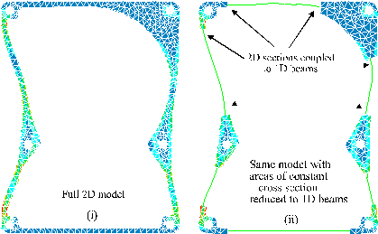
Figure 4: Sample application of 2D to 1D coupling
The process of joining entities of different geometric dimension is known as multi (or mixed) dimensional coupling. Figure 4 illustrates the concept, and it is seen that there is a marked reduction in the number of elements required to carry out the analysis (each line in (ii) consists of 1 element).
Mc Cune [], [], concentrated on 3D-2D and 2D-1D coupling. The logical next step in the process is to reduce regions of constant cross-section in 3D solids to their 1D equivalent beam element. In order to analyse stress concentrations around discontinuities in geometry and loading, the ends of this 1D beam must then be coupled to the new surfaces created by the dimensional reduction process, Figure 5. By doing so, a marked reduction in the number of DOF required to analyse the model can be achieved without any loss of accuracy.
In this paper the coupling of a 1D beam element to a 3D continuum is described. Alhough the procedure has only been implemented for linear elements, it illustrates the concept and may be further developed into a general and robust process. The reader is introduced to the area by firstly dealing with the simple case for axial force in section 3. This will be followed by the bending moment and torsion cases in sections 4 & 5 respectively. In section 6 the shear force case will be discussed, and section 7 provides some model examples and the results from performing the coupling of the mixed dimensions. Finally sections 8 and 9 conclude the work presented and indicate the plans for further development.
Notation
| Beam Cross-Sectional Area | A |
| Beam Displacements | u, v, w |
| Beam Forces | Fx, Fy, Fz |
| Beam Rotations | x, y, z |
| Bending moments | Mx, My, Mz |
| Centroid of element face | xc, yc |
| Continuum Displacements | U, V, W |
| Moment of Inertia | I |
| Poisson's Ratio | |
| Shape functions | N |
| Shear Modulus | G |
| Stress (direct) | x, y, z |
| Stress (shear) | xy, xz, yz |
| Stress function | |
| Temperature | t |
| Young's Modulus | E |
Axial Force
The following derivation is based on an outcome of Reissner's transverse plate bending theory [] by which simple relationships are shown to be obtainable between the translational and rotational degrees of freedom in a plate and the displacements in the 3D continuum. To couple a beam and a solid, the first step is to equate the work done on either side of the interface between dimensions.
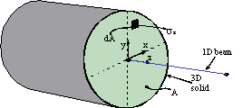
Figure 5
Equating the work done by the axial force acting on the 1D beam with the work done by the surface stresses of the 3D body at the interface, the following equation results:
... 3-1
If the 3D region is long and slender, then the axial stress is uniform over the cross-section and is given by:
... 3-2
In the 3D model, the axial displacement at any point, in terms of the nodal displacements{W} and shape functions[N], is:
W=[N]{W} ... 3-3
This implies:
... 3-4
Since this must be true for any axial force, the beam displacement w and the displacements of the 3D continuum nodes on the interface {W} must be related by:
... 3-5
Displacement compatibility between the 1D beam element and the adjacent 3D continuum elements can therefore be enforced as a multipoint constraint equation of the form
... 3-6
This can be applied in the ABAQUS commercial finite element package as a *EQUATION command [].
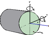
Figure 6
--------------------------------------------------------------------------------
Bending Moment
Again Reissner's relationships can be used to equate the work done on either side of the coupling interface. Considering the moment about the x-axis and equating the work done at the interface gives the following equation:
... 4-1
From simple beam theory, assuming for simplicity that the co-ordinate system is aligned with the principal axes,
... 4-2
Substituting also for the displacements in the z-direction in the 3D finite element model,
W=[N]{W} ... 4-3
On substitution:
... 4-4
This is the general solution for any type of element.
Consideration of the bending moment acting about the y-axis gives a similar equation:
... 4-5
--------------------------------------------------------------------------------
Torsion
The distribution of shear stress on the cross-section of a beam subjected to a torsional moment is commonly solved by introducing a single stress function. If a function (x,y), the Prandtl stress function, is assumed to exist such that:
... 5-1; ... 5-2
then the stress function must satisfy the differential equation:
... 5-3
where is the twist per unit length of the beam and G is the shear modulus. The stress function therefore must satisfy Poisson's equation []. A conductive heat transfer case also may be represented as a form of Poisson's equation.
Therefore, the variation of the Prandtl stress function over any cross-section can be found using the facilities available in standard finite element packages for conductive heat transfer. The shear stress on the cross-section can be inferred from the resulting temperature gradients. The cost of a 2 dimensional heat transfer analysis of the cross-section is much less than that of a 3D analysis of the stress.
The total torque generated by a given twist can be found from the torsion analysis [9] as:
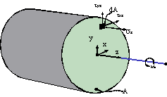
Figure 7 ... 5-4
The coupling equation is again formed by equating the work done at the interface.
On the 3D side of the interface, the work done is:
... 5-5
On the 1d side, the work done is:
... 5-6
Therefore,
... 5-7
Replacing the integral over the whole cross-section with the sum of the integrals over the element faces lying on the interface and the continuum displacements with the 3D finite element displacements:
... 5-8
The total torque Mz in response to any arbitrary twist can be found from Equation 5-4, as can the shear stresses xz and yz on each element face. Evaluating the [C] and [D] matrices reduces to summing integrals of the form:
... 5-9
The shear stress xz can be written in terms of shape functions [N] and nodal values of the stress function {} from the 2D analysis of the cross-section as:
... 5-10
so that the integral over an element face becomes:
... 5-11
where {} are the nodal temperatures found in the heat transfer analysis. The complete multipoint constraint equation can then be written in the form:
-Mzz+C1u1+ C2u2+ C3u3+.... D1v+ D2v+ D3v3....=0 ... 5-12
This equation can also be applied as a linear constraint equation in the finite element model (e.g. applied in Abaqus as a *EQUATION command). The effect of this equation is to couple the displacements of the 3D continuum nodes on the interface to the twisting rotation of the beam node such that the distribution of shear stress on the interface is the same as that given by the St. Venant torsion analysis of the beam cross-section.
--------------------------------------------------------------------------------
Shear Force
The approach in sections 3-5 may be extended to ensure the proper distribution of shear stress in response to a given shear force using an analysis of the cross-section similar to that for torsion []. The stresses on the cross-section at any point (x,y) due to a shear force Fx on the cross-section are given in terms of a stress function as

Figure 8: Shear stresses on square section resulting from a shear force
... 6-1; ... 6-2
where must obey the governing equation
... 6-3
with the boundary condition
... 6-4
on the boundary of the section.
Figure 8 illustrates the shear stress xz derived from the results of a 2D thermal analysis of the cross-section. Given the shear stresses on the cross-section, the appropriate multipoint constraint equation can be generated as before by equating the work done on both sides of the interface. This yields
... 6-5
This procedure has been demonstrated successfully for 2D - 1D coupling of beams and plates [6].
This procedure has been demonstrated successfully for 2D - 1D coupling of beams and plates [6].
--------------------------------------------------------------------------------
Results
Sample results for the cases considered are given in their respective sections below. They demonstrate the concept graphically and give an indication of the possible benefits of carrying out the reduction & coupling.
--------------------------------------------------------------------------------
AXIAL FORCE
The stress plot of the coupling for the Axial force case is shown in Figure 9 on the right. The stress is constant across the section as expected, and is the same as the analytical result.
Figure 9: Coupling for axial force
--------------------------------------------------------------------------------
BENDING MOMENT
The stress plots of the coupling for the bending moment cases are shown in Figure 10 and Figure 11 below. Again the results compare favourably with analytical calculations. Note that there is no disturbance to the stress contours at the interface between the 1D beam and the 3D solid elements.
Figure 10: Coupling for moment about x-axis (von Mises stress) Figure 11: Coupling for moment about y-axis (von Mises stress)
--------------------------------------------------------------------------------
TORSION
Figure 12: Coupling for Torsion of tubular section (max. shear stress) Figure 13: Torsion (max. shear stress)
As can be seen from the contours of maximum shear stress in Figure 12 and Figure 13 the coupling equations produce stress contours which are axisymmetric and as close to the analytic solution for a thin walled tube as can be obtained with constant stress elements and nodal averaging.
Figure 14 and Figure 15 show the von Mises stress obtained for coupling a square bar to a beam element of equivalent properties. Again there is no disturbance to the stress contours at the dimensional interface and the stresses on the interface are effectively identical to those obtained by the St. Venant torsion analysis or at sections in the interior of the 3D model. There is some disturbance at the rigidly fixed end due to the method by which the fixing was defined.
Figure 14: Torsional load (Max shear stress) Figure 15: Torsion on block
--------------------------------------------------------------------------------
Discussion
Using the procedure described here, the analysis of a slender region within a 3D solid can be reduced to a 1D analysis plus 6 simple analyses of the cross-section. These determine the stress distribution on the cross-section in response to each component of force and moment.
The cross-sectional analyses can also be used to generate 6 multipoint constraint equations linking the displacements and rotations of the beam element to the nodal displacements of the 3D continuum elements representing the material adjacent to the slender area of the model represented by the beam element. This greatly facilitates mixed-dimensional modelling, where 3D details such as joints, changes in section or loading are properly represented, but dimensionally-reduced beam elements are used to model slender parts (economically and accurately), where 3D elements are expensive and potentially ill-conditioned.
The coupling does not introduce spurious stresses at the interface, so that measures based on the implied stress jumps between the 3D and the reduced dimensional models can be used as an a posteriori estimate of the idealisation error introduced by dimensional reduction [5], [6]. The cross-sectional analyses can also be used to determine section properties for beam elements and to transfer beam force and moment results to stresses on the cross-section for visualisation.
The ideas presented here have already been applied to beam-plate-solid coupling [5] and should be extensible to the coupling of arbitrary combinations of beam, plate, shell and solid elements of any formulation.
--------------------------------------------------------------------------------
Conclusions
A general technique for coupling 1D beams to 3D continuum elements has been developed.
Only 6 multipoint constraint equations are required to couple the 1D and 3D elements at the interface between dimensions.
The coupling does not introduce any errors at the interface between dimensions.
The technique should greatly facilitate appropriate mixed-dimensional modelling of structures containing slender parts and 3D details.
- NAFEMS. (1996) How to integrate CAD and analysis, CAD/FE Integration working group, Glasgow.
- Bridgett S.J., "Detail Suppression of Stress Analysis Models", PhD thesis, The Queen’s University of Belfast, November 1997.
- Blacker T., Sheffer A., Clements J., Bercovier M., "Using Virtual Topology to Simplify the Mesh Generation Process", Proceedings of 1997 joint
- ASME/ASCE/SES summer meeting, Evanston, USA, published in American Society of Mechanical Engineers, AMD, Vol. 220, 1997, pp 45-50.
- Donaghy R.J., "Dimensional Reduction of Stress Analysis Models", PhD thesis, The Queen’s University of Belfast, May 1998.
- McCune R.W., "Mixed Dimensional Coupling and Error Estimation in Finite Element Stress Analysis", PhD thesis, The Queen’s University of Belfast, March 1998.
- Armstrong, C.G., Bridgett, S.J., Donaghy, R.J., McCune, R.J., McKeag, R.M. and Robinson, D.J., "Techniques for Interactive and Automatic Idealisation of CAD Models", 6th International Conference on Numerical Grid Generation in Computational Field Simulation, London, July 1998.
- Reissner E., "On Bending of Plates", Quarterly of Appl. Math., Vol. 5, 1947, pp 55-68.
- Hibbitt, Karlsson & Sorenson Inc., ABAQUS / Standard Users Manual, 1997, pp20.2.1-1.
- Timoshenko S.P., Goodier J.N., "Theory of Elasticity", 3rd edition, McGraw-Hill, New York, 1970, pp 291-349.
- Timoshenko S.P., Goodier J.N., "Theory of Elasticity", 3rd edition, McGraw-Hill, New York, 1970, Art 128.
